Reading Notes on Elements of Causal Inference
Table of Contents
- Preface
- Section 1 Statistical and Causal Models
- Section 2 Assumptions for Causal Inference
- Section 3 Cause-Effect Models
- Section 4 Learning Cause-Effect Models
- Section 5 Connections to Machine Learning I
- Section 6 Multivariate Causal Models
- Citation
Preface
This note reflects my personal understanding of Elements of Causal Inference by Jonas Peters, Dominik Janzing, and Bernhard Schölkopf, where I include selected quotations and figures from the book to help organize key ideas. Readers interested in full details should refer to the original text.
Section 1 Statistical and Causal Models
This section aims to let readers know that causal models are different and lead to harder inference problems, compared to statistical models/probabilistic models.
Terminologies
| Term | Alias | Definition |
|---|---|---|
| Probabilistic model | Statistical model | A model that represents (learns and infers) the joint distribution of random variables. It is related to two processes: probabilistic learning and probabilistic reasoning. |
| Probabilistic learning | Statistical learning | The process of learning a probabilistic model, including its structure and parameters. |
| Probabilistic reasoning | Probabilistic inference Note: Some papers may use “inference” to refer to learning and reasoning. Here, we use “inference” to refer to reasoning only. | The process of inferring joint distributions, marginal distributions, and conditional distributions. |
| Correlation | Statistical dependency | Different from independence. |
| Causal model | A model that represents the causal relationships between random variables. That is, a model that learns the causal relationships between random variables and can be used to do causal reasoning. | |
| Causal learning | The process of learning a causal model, including its structure and parameters. | |
| Causal structure | The graphical structure of a causal model. The problem of studying whether the causal structure can be recovered from the joint distribution is called “structure identifiability”. The problem of estimating the causal structure from empirical implications is called “structure learning/causal discovery/structure identification”. | |
| Causal reasoning | Causal inference | The process of inferring joint distributions, marginal distributions, conditional distributions, and distributions under interventions or distributional changes. |
| Joint distribution | Observational distribution | Different from interventional distribution. |
Relationships
Correlation does not imply causation.
If \(X\) is correlated with \(Y\), there might not be a direct causal relationship between X and Y. Instead,
The dependency between X and Y admits several causal explanations.
One of my favorite examples is:
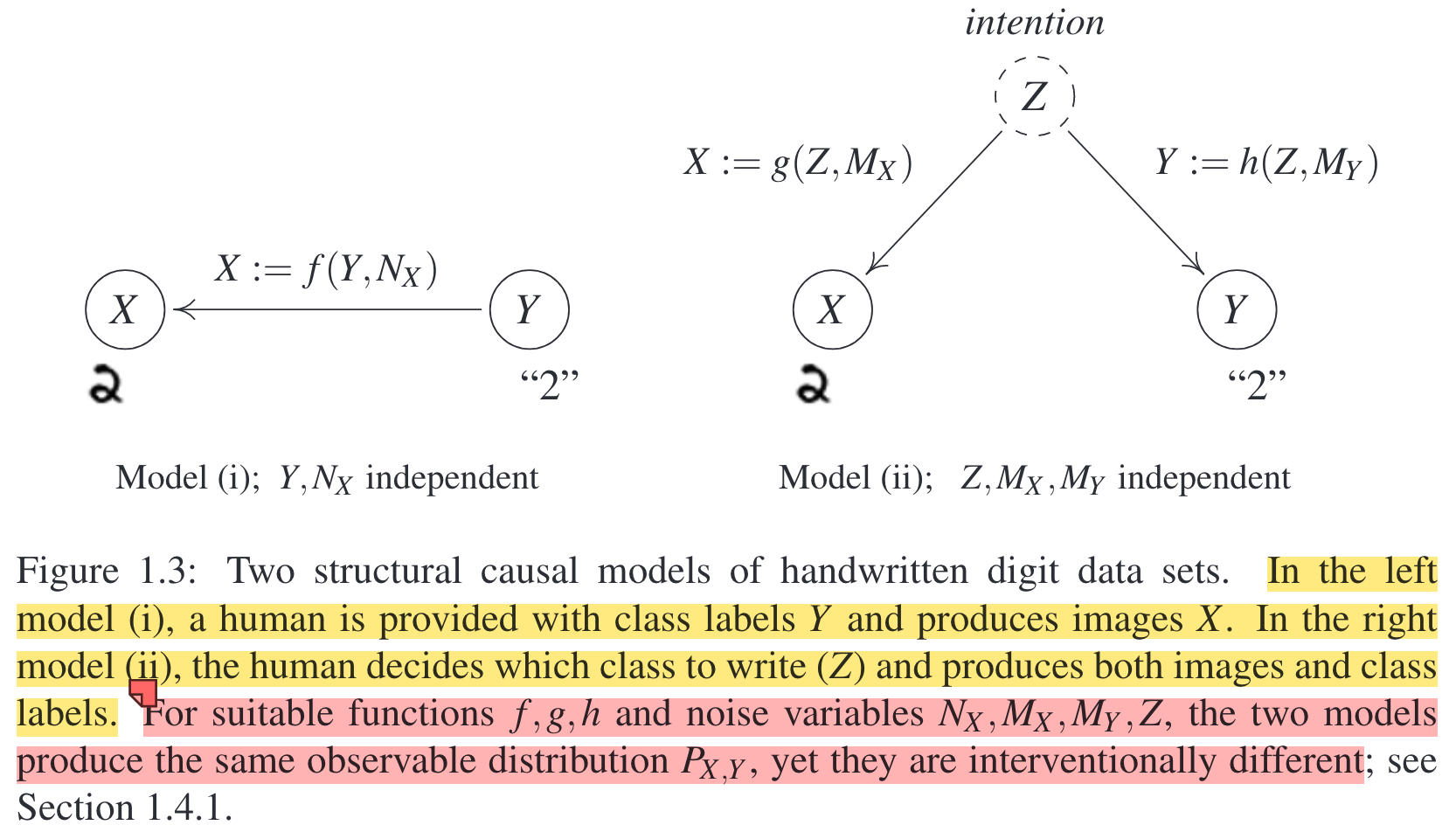
From this example, we can see that:
- Multiple causal structures may account for the correlation between \(X\) and \(Y\).
- Different causal structures may lead to the same joint distributions, yet different interventional distributions.
- \(X\) and \(Y\) become independent if we condition on \(Z\) in the right-hand figure, because the image and the label share no information that is not contained in the intention.
In fact, the following principle guarantees the existence of a causal explanation.

More specifically, borrowing concepts from Section 6, we have:
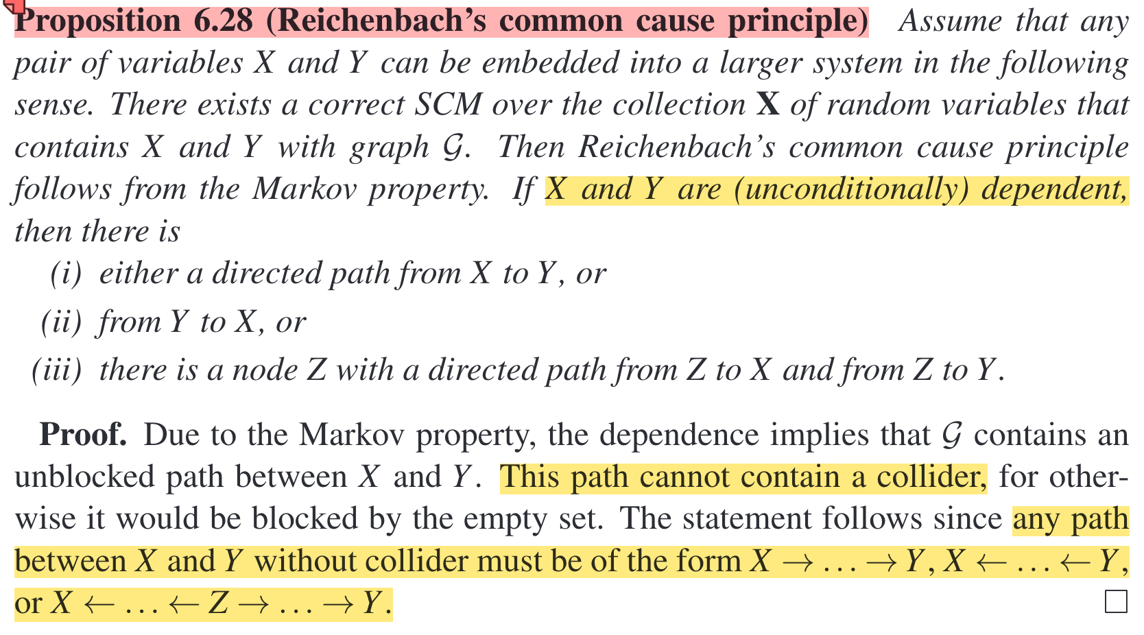
That is, if \(X\) and \(Y\) are dependent, then on the path between \(X\) and \(Y\), there cannot be a collider. Consequently, the path must be one of the forms, which validates the existence of \(Z\).
A causal model entails a probabilistic model.
This is because the causal model can not only be used to infer joint distributions, but also to infer interventional distributions.
Section 2 Assumptions for Causal Inference
This section aims to let readers know the underlying assumptions/principles used in causal inference—causal mechanisms are invariant.
Principles of independent mechanisms
(1) The mechanism of a variable, i.e., the conditional distribution of each variable given its causes, does not inform or influence the other conditional distributions. In case we have only two variables, this reduces to an independence between the cause distribution and the mechanism producing the effect distribution.
(1’) In other words, the causal generative process of a system’s variables is composed of autonomous, modular, invariant modules that do not inform or influence each other.
Suppose we have estimated the joint density \(p(a,t)\) of the altitude \(A\) and the average annual temperature \(T\) of a sample of cities in some country.
How can we utilize this principle to decide which of the two structures—\(T \to A\) and \(A \to T\)—is the causal one? That is, which of the two factorizations—\(p(a,t) = p(a\mid t)p(t)\) and \(p(a,t) = p(t\mid a)p(a)\)—is meaningful?
Approach 1: Do interventions Intervening on \(A\) changes \(T\), while intervening on \(T\) does not change \(A\). Hence, \(A \to T\) is the causal one.
Approach 2: Change cause distributions Changing \(p(a)\) from that in China to that in the US does not influence \(p(t|a)\). Hence, \(p(a,t) = p(t|a)p(a)\) is the meaningful one.
(2) Given any mechanism, the noise is independent of the cause variables.
(3) Noises for different mechanisms are jointly independent.
Moreover, we will know in Section 6 that:
(4) The mechanism of a variable is invariant to interventions as long as the intervention is not conducted on this variable.
Formally,


In summary, causal mechanisms are invariant to other conditional distributions or the cause distributions.
Section 3 Cause-Effect Models
This section aims to let readers know a few concepts: SCM, interventions, and counterfactuals, in the context of two variables.
Structural causal models that contain only two variables

A more general definition is: a structural causal model, sometimes called a structural equation model, has all dependencies generated by functions that compute variables from other variables, and all noise terms are jointly independent.
How to sample data from an SCM? Given noise distributions \(N_C, N_E\) and the function \(f_E\), we first sample noise values \(N_C, N_E\), and then evaluate (3.1) followed by (3.2). From this, we can see that an SCM entails a joint distribution \(P_{C,E}\) over \(C\) and \(E\).
SCMs are one type of causal models.
Interventions
Hard interventions set a variable to a fixed value, e.g., \(do(E:=4)\).
Soft interventions keep a functional dependency but may change the noise distribution or the function, e.g., \(do(E:=g_E(C, \tilde{N}_E))\).
Intervention is different from conditioning. More specifically, intervening on a variable \(X\), e.g, setting it to a fixed value \(x\), is different from including \(X=x\) as the condition. The interventional distributions are sometimes identical to the conditional distributions. A detailed discussion will be presented later.
Counterfactuals
A counterfactual question looks like “What would have happened had the doctor administered treatment \(T=0\)?”
Typically, the counterfactual distribution is computed after certain observations have been made. Computing the counterfactual distribution involves two steps—conditioning + interventions:
- Condition on observations to update the distributions over noise variables;
- Do interventions.
Finally, the counterfactual distribution looks like \(P^{\mathcal{C} \mid B=1, T=1; do(T:=0)}\).
Section 4 Learning Cause-Effect Models
This section aims to let readers know under which assumptions the structure (i.e., \(X \to Y\) or \(Y \to X\)) can be recovered from the joint distribution (structure identifiability), and methods that estimate the structure from a finite data set (structure identification).
Structure identifiability

This theorem tells us that if the joint distribution \(P_{X, Y}\) admits a linear causal model mapping \(X\) to \(Y\) with non-Gaussian additive noise, then there does not exist a linear causal model mapping \(Y\) to \(X\) with non-Gaussian additive noise because in this case, \(N_X\) will be dependent of \(Y\), which does not satisfy the principle of independence. That is, under the assumption of linear causal models with non-Gaussian additive noise, only one of the structures, i.e., either \(X \to Y\) or \(Y \to X\), will hold.
Below is an example to clarify this:
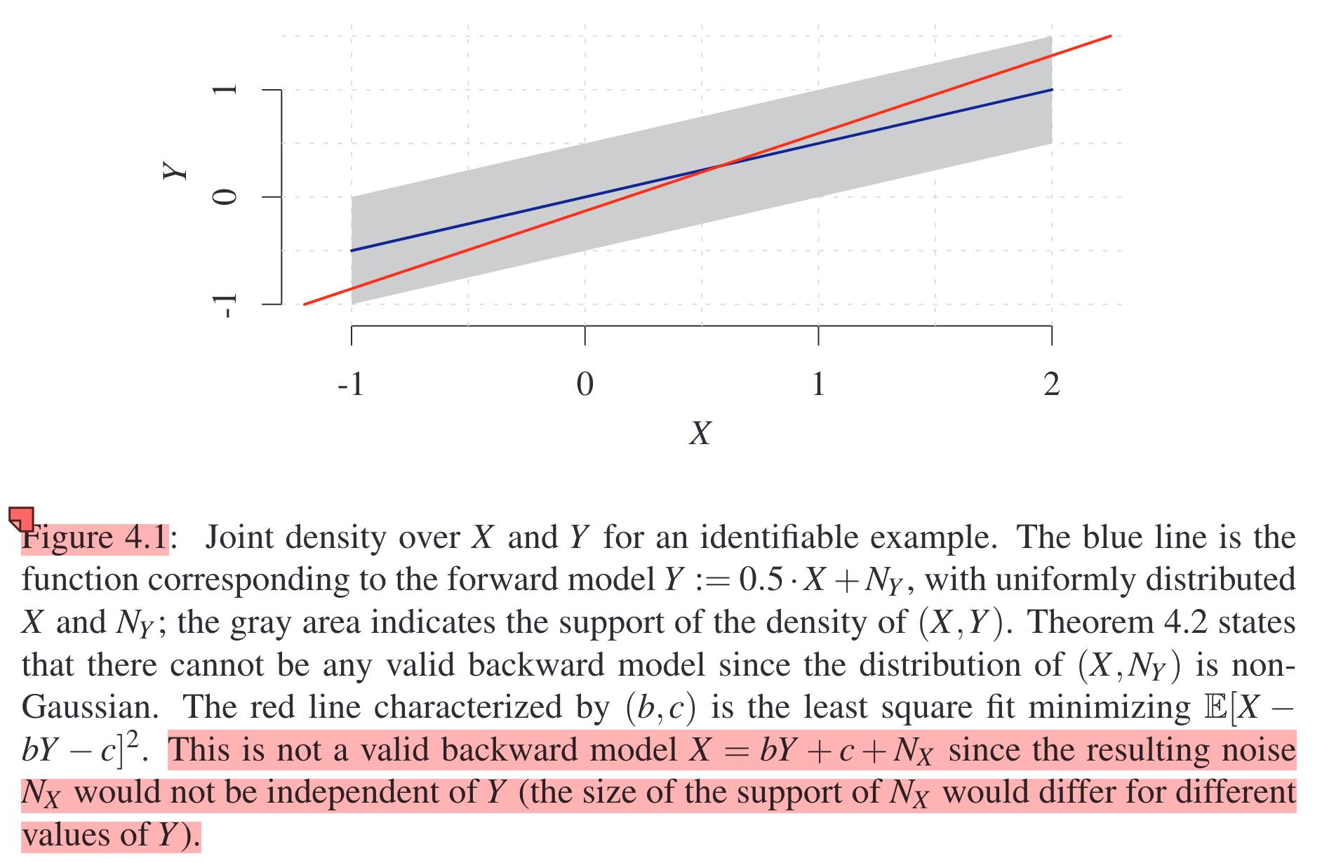

A similar theorem holds for ANMs. That is, under the assumption of nonlinear additive noise causal models, only one of the structures, i.e., either \(X \to Y\) or \(Y \to X\), will hold.
Structure identification
Structure identifiability tells us that under certain assumptions, only one of the structures holds. Next, structure identification will tell us which specific structure holds.
Goal: Decide the causal model is \(Y = f_Y(X) + N_Y\) or \(X = f_X(Y) + N_X\).
Approach 1: Independence test on residuals

Below is an example:
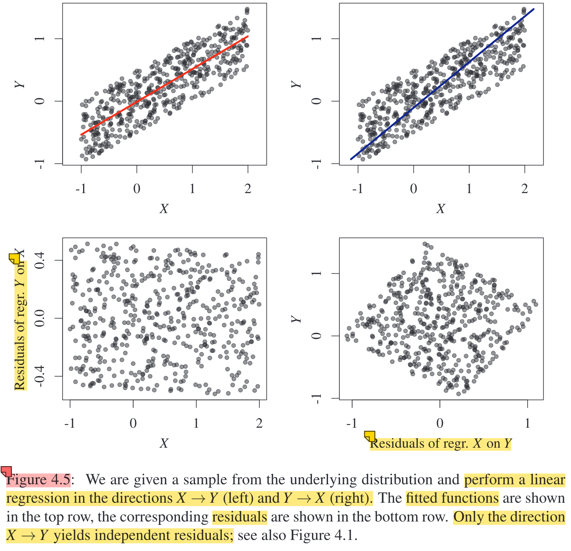
Approach 2: Maximum likelihood-based approach~
- Do regressions for both directions.
- Select the model with the larger likelihood (smaller variance).
Section 5 Connections to Machine Learning I
Semi-Supervised Learning (SSL)
SSL refers to learning with labeled data \((x,y)\) and unlabeled data \(x\). SSL does not help (i.e., tells us nothing about \(P_{Y|X}\)) when \(X \to Y\). This is because the unlabeled data \(x\) reveals more information about \(P_X\); however, \(P_X\) and \(P_{Y|X}\) are independent when \(X \to Y\). Note: It doesn’t mean knowing more about \(P_X\) is helpless; on the contrary, it may help us to better estimate \(Y\) in the sense of obtaining lower risk.
Covariate Shift
Covariate shift refers to the scenario where \(P_X\) is changed while \(P_{Y\mid X}\) remains the same. This scenario is only justified when \(X \to Y\).
Section 6 Multivariate Causal Models
Graph terminology
- A graph \(\mathcal{G}_1=\left(\mathbf{V}_1, \mathcal{E}_1\right)\) is called a subgraph of \(\mathcal{G}\) if \(\mathbf{V}_1=\mathbf{V}\) and \(\mathcal{E}_1 \subseteq \mathcal{E}\); we then write \(\mathcal{G}_1 \leq \mathcal{G}\). If additionally, \(\mathcal{E}_1 \neq \mathcal{E}\), then \(\mathcal{G}_1\) is a proper subgraph of \(\mathcal{G}\).
- Three nodes are called an immorality or a v-structure if one node is a child of the two others that themselves are not adjacent.
- An (undirected) path in \(\mathcal{G}\) is a sequence of (at least two) distinct vertices \(i_1, \ldots, i_m\), such that there is an edge between \(i_k\) and \(i_{k+1}\) for all \(k=1, \ldots, m-1\). If \(i_{k-1} \rightarrow i_k\) and \(i_{k+1} \rightarrow i_k, i_k\) is called a collider relative to this path. If \(i_k \rightarrow i_{k+1}\) for all \(k\), we speak of a directed path from \(i_1\) to \(i_m\) and call \(i_1\) an ancestor of \(i_m\) and \(i_m\) a descendant of \(i_1\).
- \(\mathcal{G}\) is called a directed acyclic graph (DAG) if all edges are directed and there is no directed cycle.
- d-separation
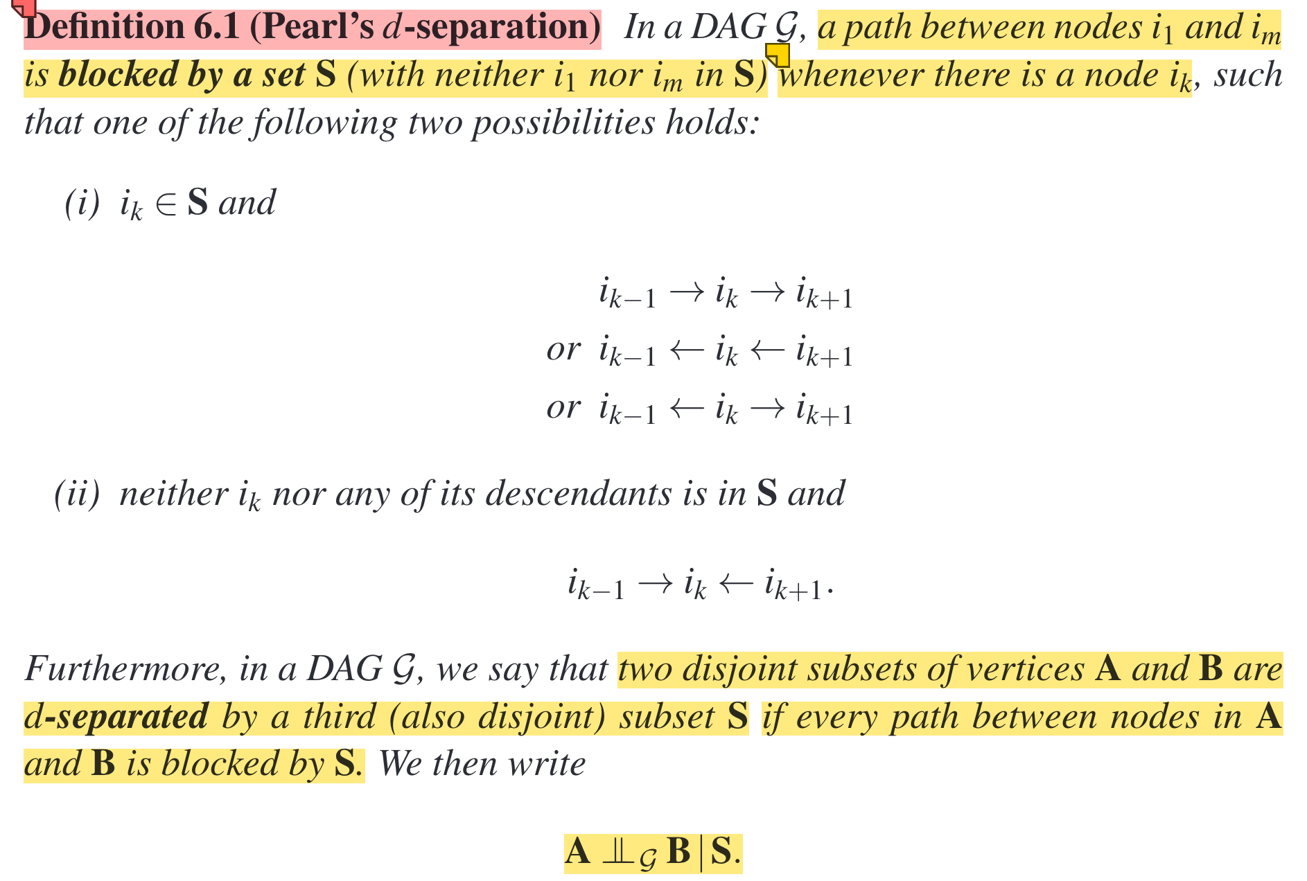
How to decide when \(i_k\) should (not) be put in \(S\)?
- In the first three cases, given \(i_k\), \(i_{k-1}\) and \(i_{k+1}\) will be conditionally independent. Therefore, if we want to block \(i_{k-1}\) and \(i_{k+1}\), making them independent, then we need to put \(i_k\) into \(S\). An example for the third case is:
| \(i_{k-1}\) | \(i_{k}\) | \(i_{k+1}\) |
|---|---|---|
| The road is wet. | It is raining. | People are using umbrellas. |
- In the last case, \(i_{k-1}\) and \(i_{k+1}\) are originally independent. Given \(i_k\), however, \(i_{k-1}\) and \(i_{k+1}\) will be dependent. Therefore, if we want to block \(i_{k-1}\) and \(i_{k+1}\), making them independent, then we cannot put \(i_k\) into \(S\). An example for the last case is:
| \(i_{k-1}\) | \(i_{k}\) | \(i_{k+1}\) |
|---|---|---|
| It is raining. | The road is wet. | The water truck passes by. |
Structural causal models
Definition.


SCM = Structural equations + Jointly independent noise distributions
Properties.

This proposition shows that: An SCM entails a joint distribution.
Proof sketch: It is easy to see that, by substituting variables in an appropriate order, we can finally obtain \(X_j = g_j(\text{noise variables of } X_j\text{'s ancestors})\). That is, \(X_j\) is a function of noise variables. By applying the transformation of densities, we can obtain \(p_X\) from \(p_N\).
Remark: One SCM gives you one joint distribution. But, one joint distribution may be compatible with many SCMs, especially if you allow complex or complete graphs. This reflects a common theme in causality: The forward process (SCM → distribution) is deterministic. The inverse problem (distribution → SCM) is non-identifiable without extra assumptions (like sparsity, acyclicity, additive noise, etc.).
Interventions
Definition.

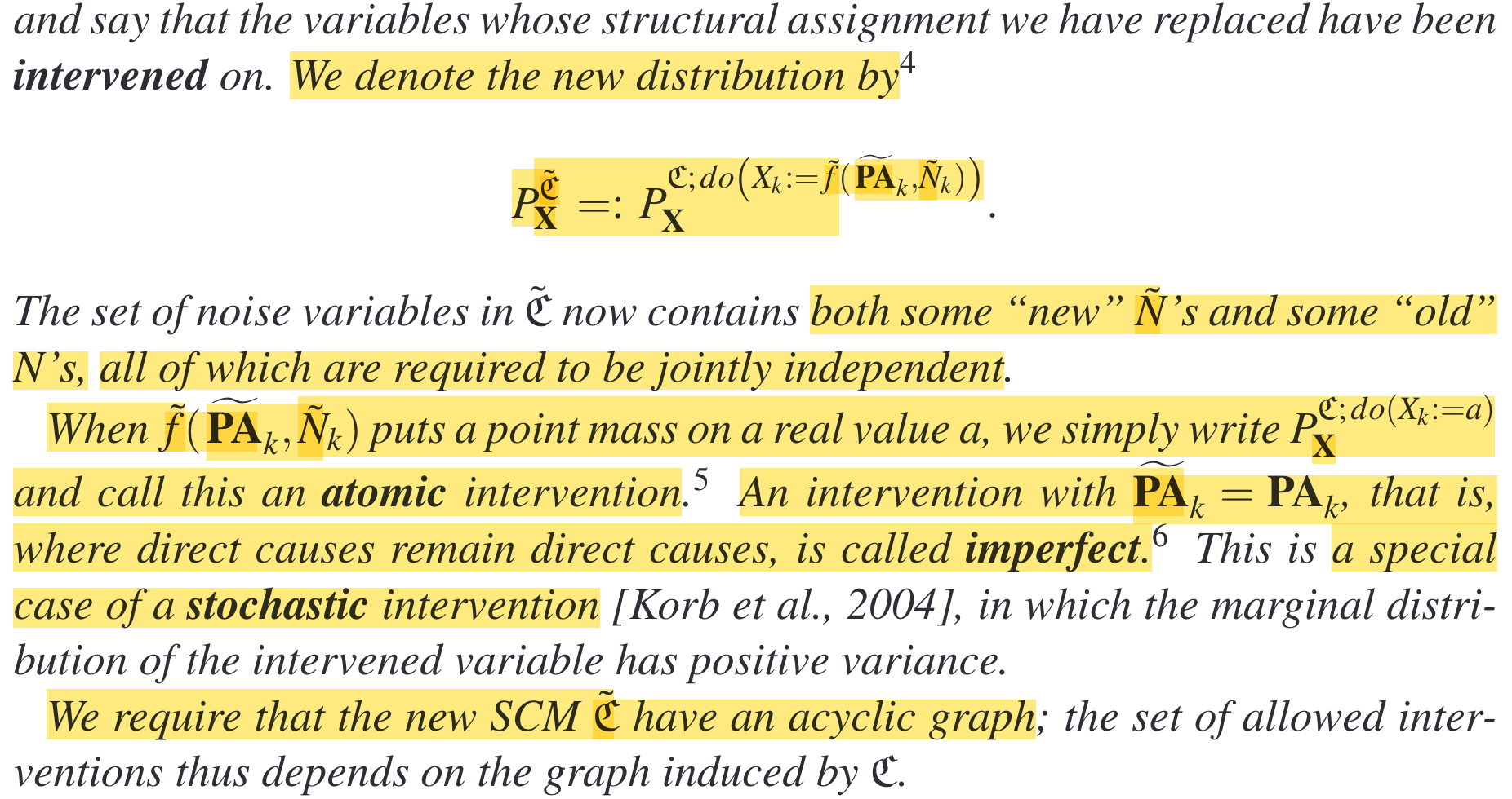
Remarks:
- If we want to intervene on \(X_k\), i.e., we want to define a new structural equation for \(X_k\), we can modify three things: 1) the function, 2) the parents, and 3) the noise.
- If we modify the parents, we need to keep in mind that we cannot introduce a cycle in the graphical structure. That is, the structure should remain as a DAG.
- If we modify the noise, we need to keep in mind that all noises should remain jointly independent.
Total causal effect.

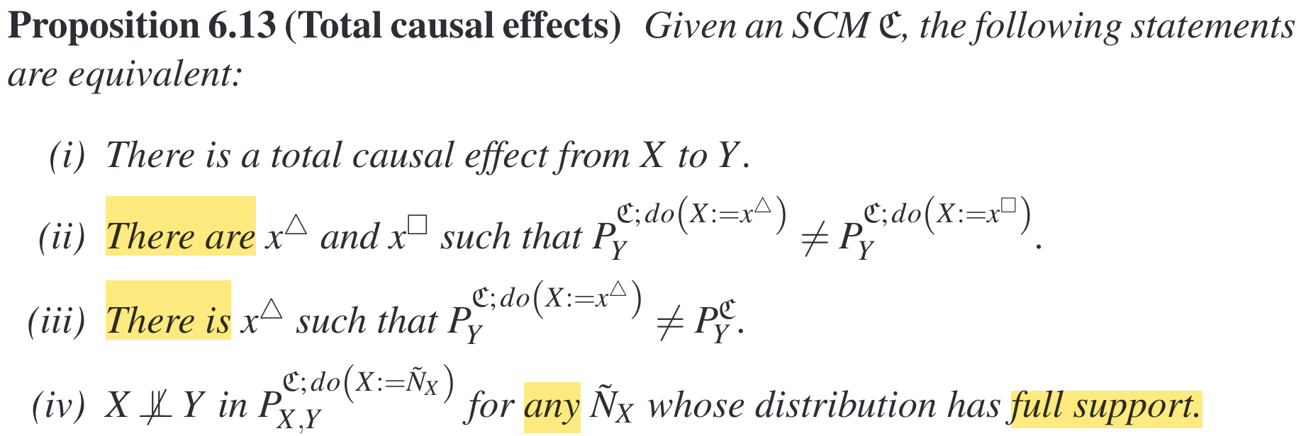
Remarks:
- These four arguments are equivalent, all of them pointing to one fact—whether there is a real value of \(X\) that can affect \(Y\). What differs is that the first three arguments use the language of \(\exists\), while the last argument uses the language of \(\forall\).
- If there is a directed path from \(X\) to \(Y\), then in terms of the graph terminology, \(X\) is called an ancestor of \(Y\); and in terms of the causal learning, \(X\) is called a cause of \(Y\).
- If there is a directed edge from \(X\) to \(Y\), then in terms of the graph terminology, \(X\) is called a parent of \(Y\); and in terms of the causal learning, \(X\) is called a direct cause of \(Y\).
- However, the fact that \(X\) is a cause of \(Y\), i.e., \(X\) is an ancestor of \(Y\), i.e., there is a directed path from \(X\) to \(Y\), does not necessarily mean there is a total causal effect from \(X\) to \(Y\). See the following proposition.

This is because a system can be constructed in such a way that the positive and negative effects cancel out; thus, the total causal effect is 0, and there is no total causal effect.
Randomized trials. Randomized trials refer to the experimental setup where each patient is given a random treatment/the treatment is randomly assigned. Randomized trials can be seen as a mathematical construct for interventions. In theory, in all treatment groups, any factor (e.g., age) other than the treatment itself has the same distribution across the groups. In practice, in all treatment groups, any factor (e.g., age) other than the treatment itself has a similar distribution across the groups. The benefit of using randomized trials is that we can estimate the average causal effect (ACE) for binary variables—\(\mathbb{E}[Y\mid do(X=1)]−\mathbb{E}[Y\mid do(X=0)]\)—directly by comparing outcomes between groups.
Simpson’s paradox.
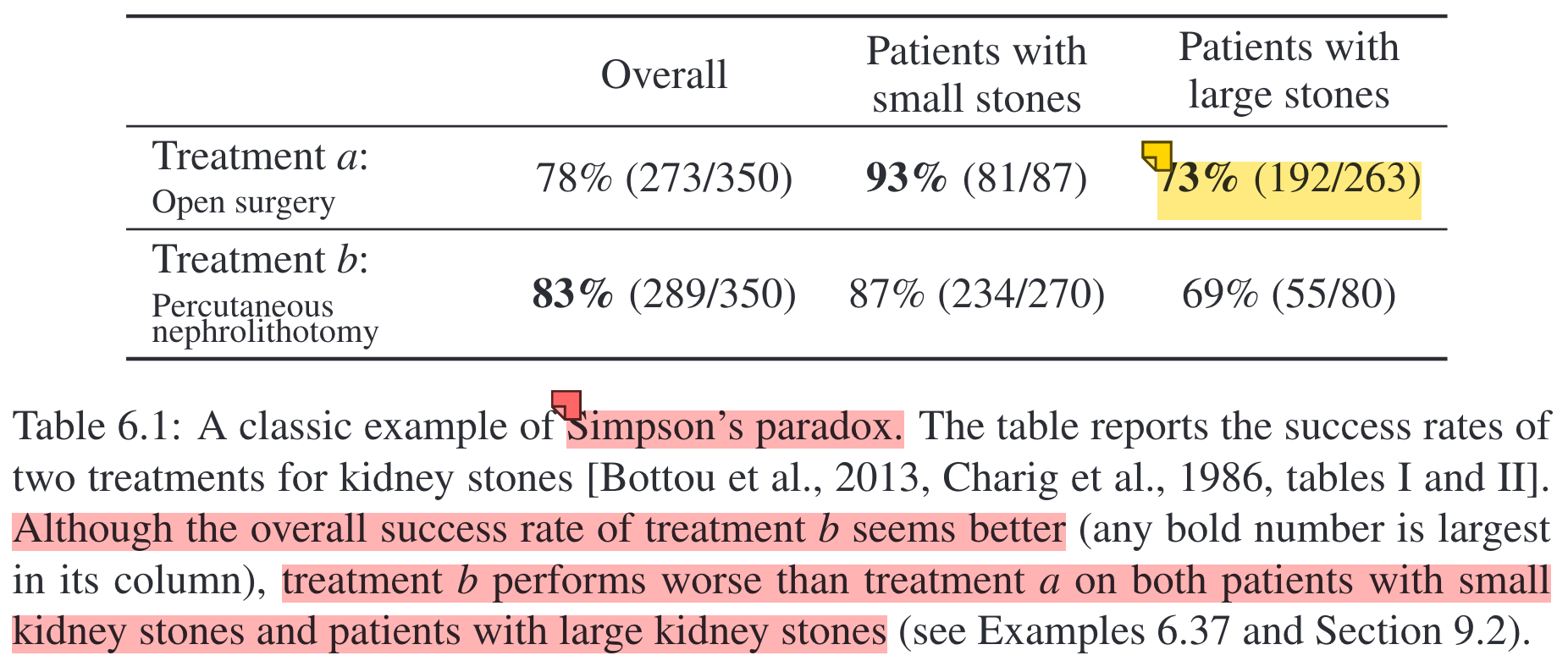
Analysis: Larger stones are more severe than small stones, and treatment had to deal with many more of these difficult cases (even though the total number of patients assigned to \(a\) and \(b\) is equal). This is why treatment \(a\) can look worse than \(b\) on the full population but better in both subgroups.
Intervention vs. conditioning. [Below incorporates some content from Section 6.6]
Difference between intervention and conditioning:
Intervention on \(X\) will affect the distributions of all variables for which the total causal effect from \(X\) to them is nonzero. The necessary (but not sufficient) condition for a nonzero total causal effect from \(X\) to \(Y\) is that there exists a directed path from \(X\) to \(Y\). Conditioning on \(X\) will affect the distributions of all variables that are correlated with \(X\).
When does intervention = conditioning:
Intervention is the same as conditioning for variables that do not have any parents. Why? Using the principle that mechanisms of generating \(X_j\) are invariant under interventions on \(X_k\), we have


When does intervention != conditioning:
Intervention is not the same as conditioning when there exists a confounder. Why?
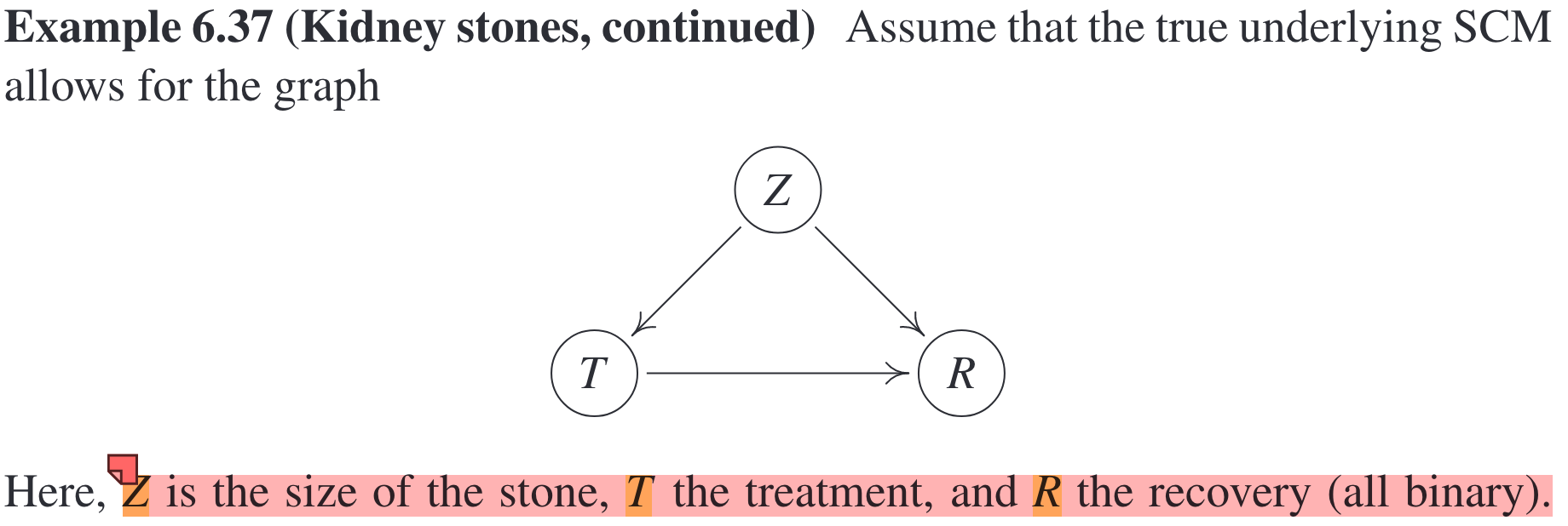
In this three-node example, intervention distribution and conditional distribution are computed as follows.
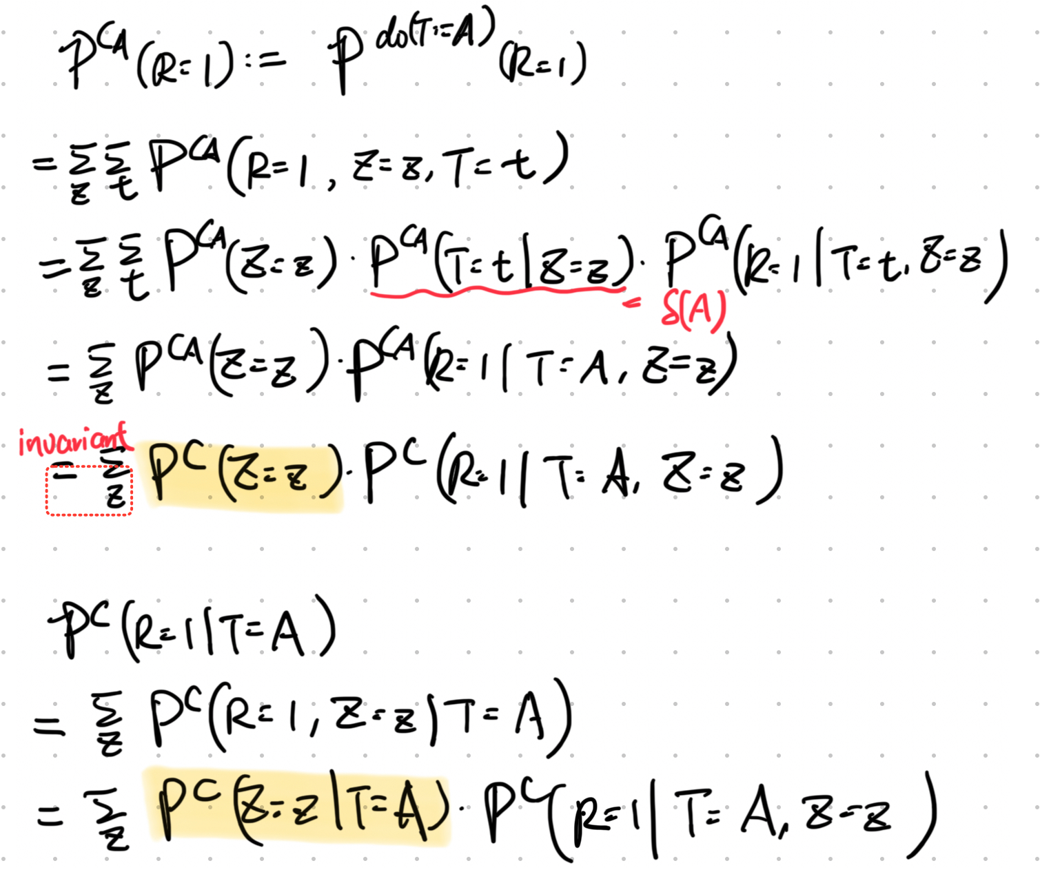
That is, they only differ in the first term. And this difference originates from the existence of \(T\)’s parent, the confounder, \(Z\). In this case, where the intervention distribution is not the same as the conditional distribution, we say the causal effect from \(T\) to \(R\) is confounded.
How to transfer intervention to conditioning:
Introduce intervention variables.
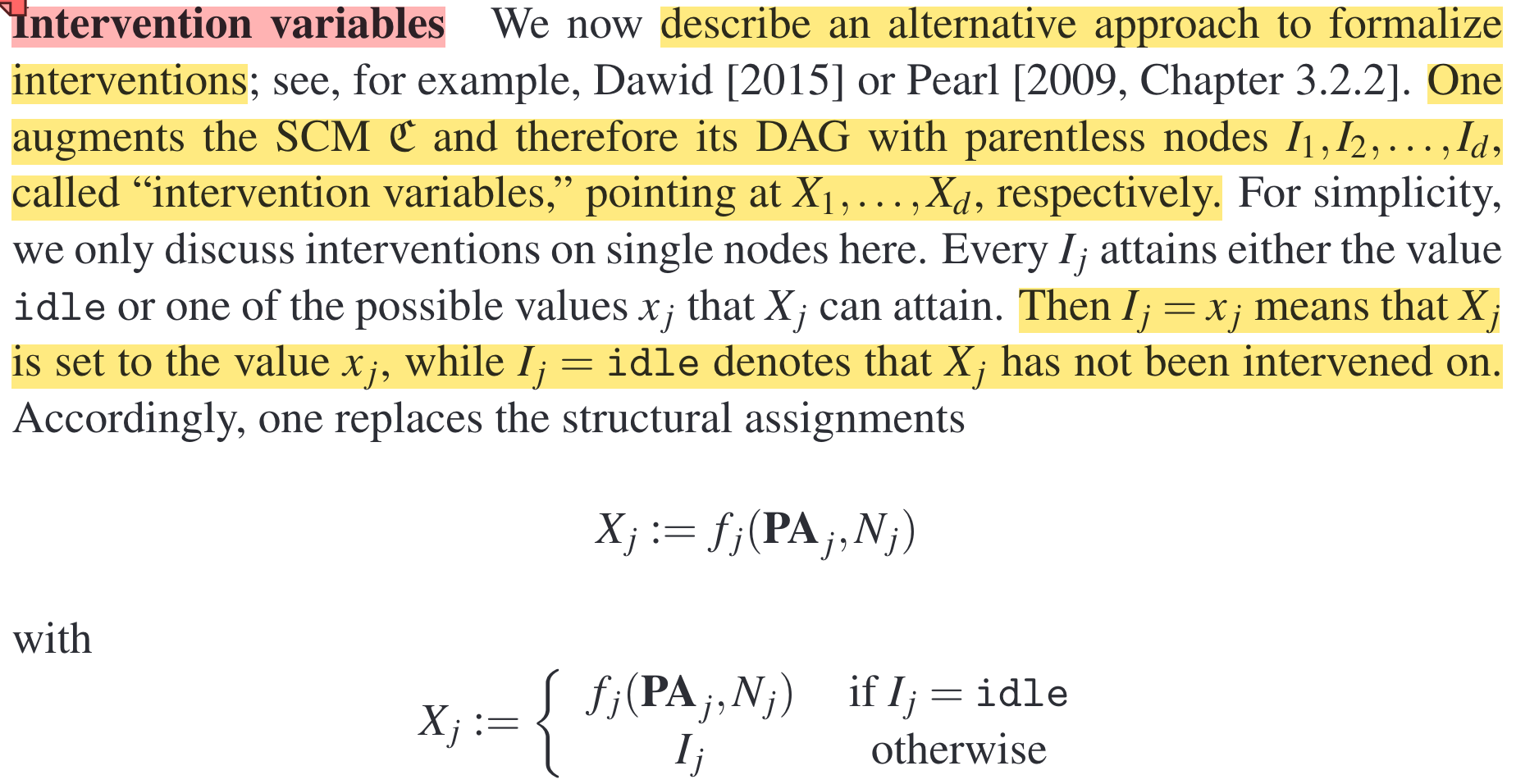
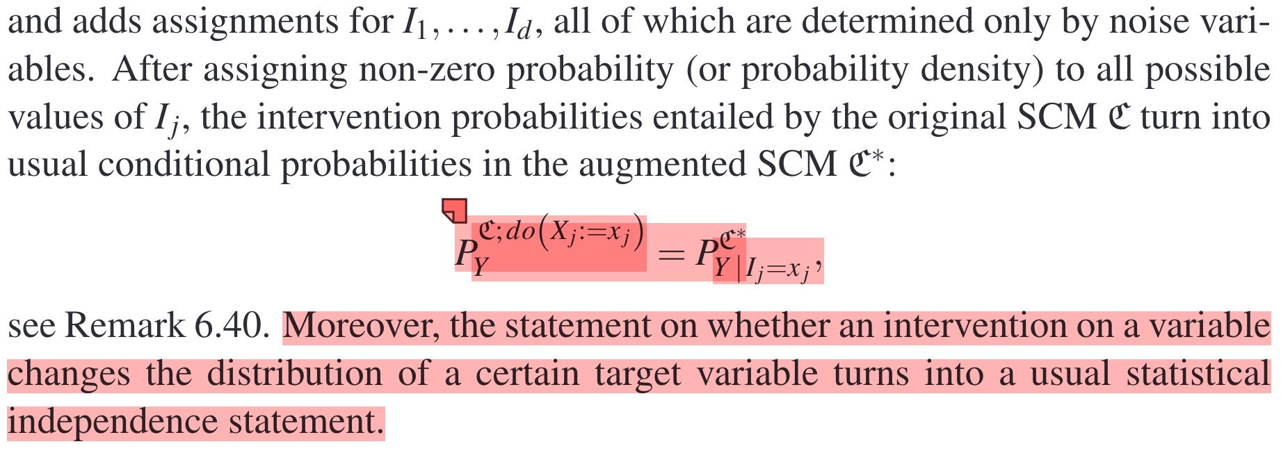
Computing interventional probabilities.
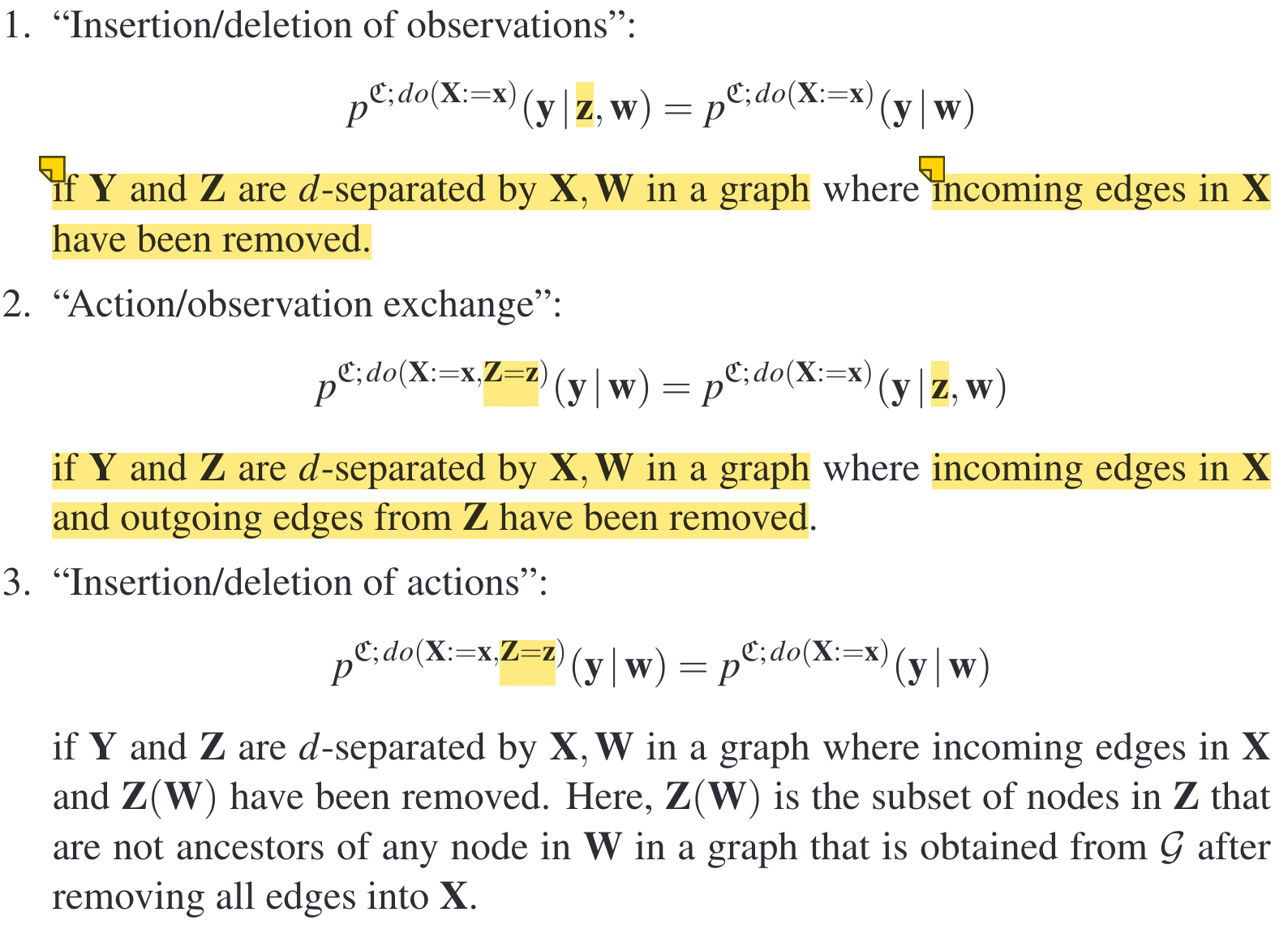
Do-calculus consists of three rules that convert the computation of interventional probabilities into the computation of observational probabilities.
Counterfactuals
Definition.
A counterfactual statement corresponds to updating the noise distributions of an SCM (by conditioning)—\(P_{N \mid X_{1:j}=x}\)—and then performing an intervention.
Remarks:
- Conditioning on \(x\) not only fixes \(X_{1:j}\) as \(x\), but also changes the values of \(X_{1:j}\)’s descendants.
- Interventions are performed after conditioning. The values specified in interventions may cover those inferred in conditioning.
- It’s possible that two SCMs correspond to the same joint distributions and intervention distributions but entail different counterfactual statements.
We can think of interventional statements as a mathematical construct for (randomized) experiments. For counterfactual statements, there is no comparable correspondence in the real world.
Markov property, faithfulness, and causal minimality
Definition.
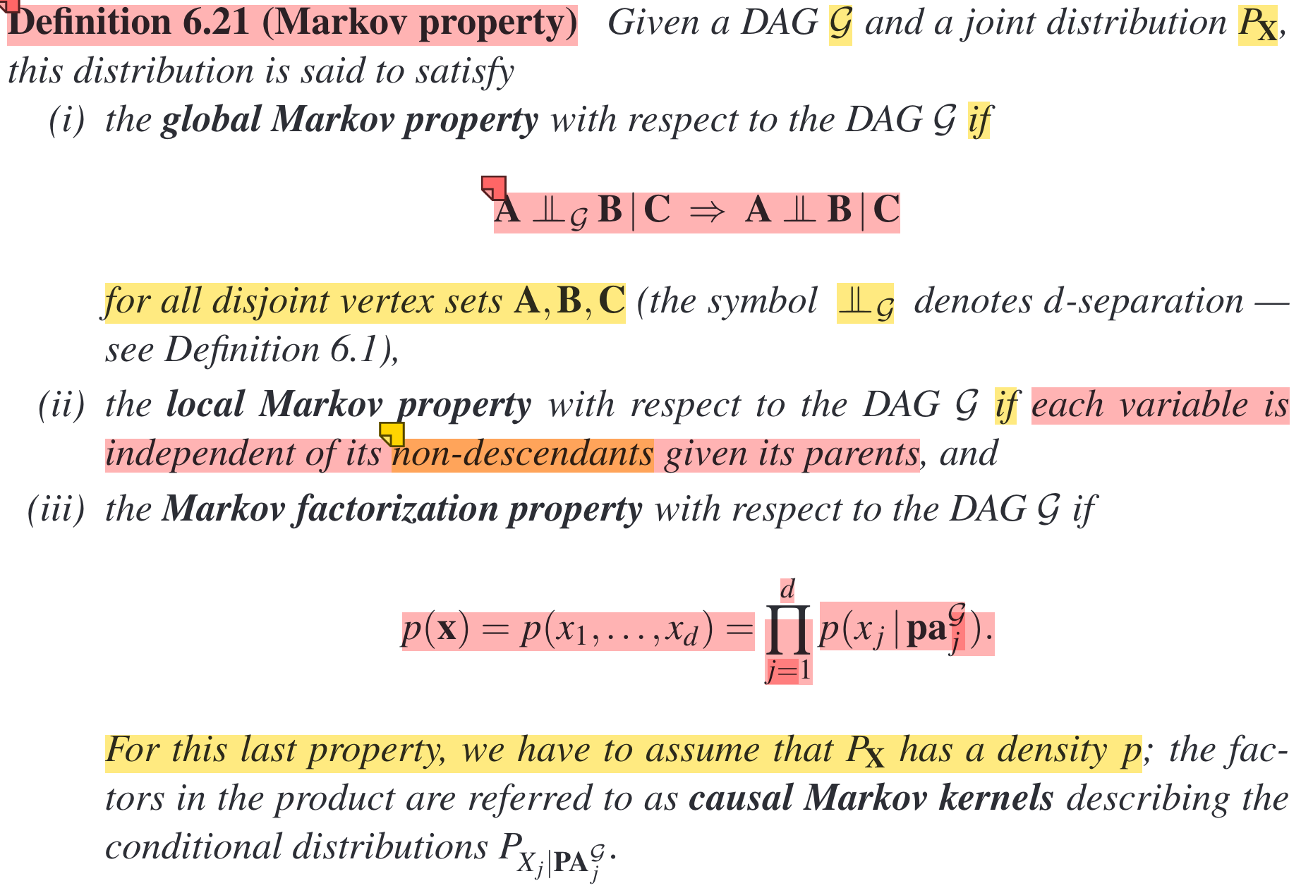

An intuitive understanding of why the three statements are equivalent: This is because they all point to the same thing, i.e., the variable distributions are built following the graph structure. Specifically, if \(A_{1:n}\) are parents of \(B\) in the graph, then the distribution of \(B\) should be constructed upon those of its parents. Recall the structural equation in SCM.
A distribution entailed from an SCM is Markovian with respect to the graph of the SCM.
On a high level, as long as the variable distributions are constructed following the graph structure, then we can say the joint distribution is Markovian w.r.t. the graph.
Markov equivalence.


In summary, if two DAGs have the same skeleton and the same v-structures, then they have the same d-separations. If they have the same d-separations, then they are Markov equivalent.
Same skeleton + v-structures -> Same d-separations -> Markov equivalence
Causal graphical models
| Causal model | Definition | Entailed distributions | |
|---|---|---|---|
| Structural causal model | = a set of structural equations + a jointly independent noise distribution | Joint distributions, intervention distributions, and counterfactual statements | |
| Causal graphical model | = a graph structure + an observational distribution that is Markovian w.r.t. the graph | Joint distributions and intervention distributions | The motivation for defining a causal graphical model: For defining intervention distributions, it usually suffices to have knowledge of the observational distribution and the graph structure. |
SCMs contain strictly more information than causal graphical models. That’s why we primarily work with SCMs.
Citation
Please cite this work as:
Chen, Weixin. Reading Notes on “Elements of Causal Inference”. Personal Blog (September 2025). https://chenweixin107.github.io/2025/09/05/causal-inference-notes.html
Or use the BibTeX citation:
@article{chen2025causalnotes,
  title   = {Reading Notes on "Elements of Causal Inference"},
  author  = {Chen, Weixin},
  journal = {chenweixin107.github.io},
  year    = {2025},
  month   = {September},
  url     = {https://chenweixin107.github.io/2025/09/05/causal-inference-notes.html}
}